This is the third article in a three-part series. You can read the first and second articles here.
The focus of this article is to understand neural network around what it is, why it is an important learning algorithm, how it is applied, its extensions & variations, etc.
A neural network is actually a pretty old idea. It is an attempt to mimic the behavior of the human brain. With the following understanding of the same,
- Human brain solves problems with large clusters of interconnected neurons.
- Each neural unit is connected with many others.
- The links will be having an effect on the activation of the connected neural units.
- Each neuron will also have an aggregation (computation) function, which will aggregate all the signal/information passed through the interconnections.
- The same will be passed on to other connected neurons.
This entire system is self-learned, through the evolution of learning. Each small learning activity performed by us from childhood will result in triggering of billions of interconnections among millions of neurons.
It is precisely this behavior that the neural network tries to mimic. It attempts to create similar interconnected artificial neurons (also called perceptrons).
Though this idea has been there for a long time, it has fallen out of favor for a while, due to its computational requirements. Such massive computational resources were not available in those days. But its resurgence in the recent past is largely due to the availability of such computational resources at disposal.
Background:
As looked at earlier in Part 2, logistic regression can be used as both simple linear classifier and complex non-linear classifier.
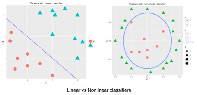
The moment we bring polynomial features (quadratic, cubic, etc.) into the feature space, we can come out with the extremely complicated non-linear classifier. But in reality, it is not easy to identify which of these polynomial features should be brought into the model. Especially when we have 100s of features available in the dataset.
For example, if we are trying to build a classification model for the risk of diabetes or hypertension based on the patient details/history. There can be hundreds of features like patient’s’ age, height, weight, etc.
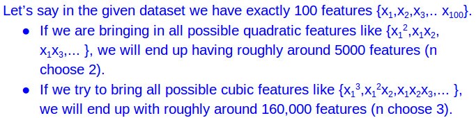
With these numbers, it is very clear that we cannot manually pick and choose which are the best features to be brought into the model. Especially when the feature space becomes so large when bringing in polynomial features.
Hence it would be helpful if we can devise a mechanism,
- To bring in all possible combinations of these features
- Associate right set of weights with each of them
- To come out with a model that fits the data in a best possible way.
This is precisely what neural network is trying to achieve.
Model representation:
The neural network model is constructed with a set of interconnected units of artificial neurons (perceptrons). They are called logistic unit when a sigmoid activation function is used. These units are the foundation blocks of the neural network system.
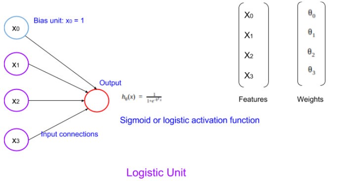
A single unit of the neural network can be visualized as shown in the picture above. As it uses a sigmoid/logistic activation function, the hypothesis function would be as shown above. Now in any given neural network, there will be a cluster/network of such units.
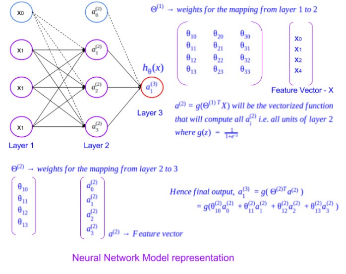
The extension from a single logistic unit to the whole neural network can be visualized as below. It has multiple layers. An input layer, an output layer and a set of hidden layers in between. When the units get interconnected across layers,
- Activation values from a given layer act as the feature vector of the successive layer.
- Each of the interconnection will have a unique weight associated with.
- As can be seen in the logistic unit representation, the set of interconnections coming into a given unit forms the weight vector for it.
- Hence the weights for the connection between layers with multiple nodes involved in both the layers results in a matrix of weights (for example layer 1 to 2 in the figure).
- Each layer has a bias unit with value 1.
- For a binary classification problem, the last layer (output layer) will have a single unit, which represents the intended output. And a multi-class classifier will have as many nodes as the number of classes.

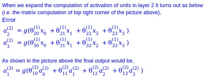
Intuitively if you try to understand, it can be seen that a neural network derives/learns features in an automatic fashion. That is the units available in all the hidden layers represent a unique derived feature. With more and more hidden layers, a number of features are automatically derived and included part of the model. At the same time, it will require a massive amount of computation, with every new layer introduced (especially with a large number of features).
Now it should be clear to some extent on,
- How neural network solves the issue of feature selection and inclusion of polynomial features in an automatic fashion.
- Why neural network has massive requirements for computational resources.
Cost Function:
As we use the logistic function in each unit, we will use the same cost function that we used for logistic regression.
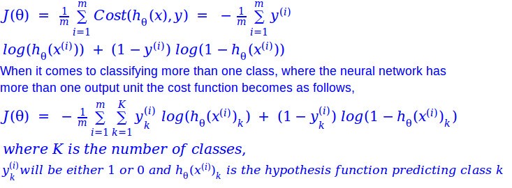
Something important to note here will be on, how to compute the classification error, where there are multiple layers involved. Logically the error in classification can be computed only in the output layer. And the same has to be propagated towards other layers until the layer next to the input layer. As it doesn’t make sense to associate an error with the input layer.
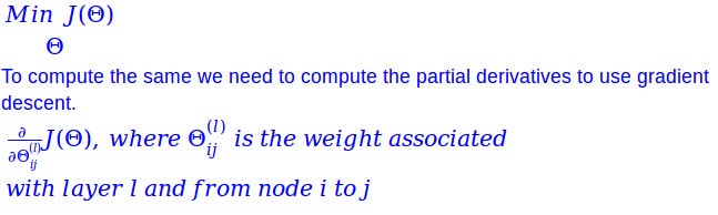
Parameter estimation:
The mechanism of parameter estimation for the neural network is complicated, with the heavy mathematics involved. Hence, the scope of this section is restricted to understanding the intuition behind the mechanism.
As with any algorithm, the parameters are estimated with an optimization object on top of the cost function.
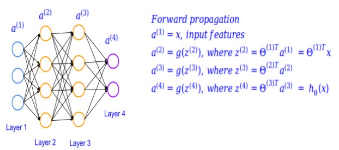
Let’s see how we can compute this. The way of estimating parameters of every layer all the way up to the output layer illustrated below is called forward propagation. Where we estimate the parameters in a given layer, from the parameters of the previous layer, and the weights of the interconnection.
But to actually estimate the parameters by minimizing the classification error, we have to use back propagation method. As the classification error can only be computed from the output layer to start with.
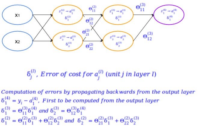
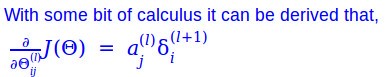
Based on the back propagation mentioned above the error from the successive layers can be used to compute these values.
As mentioned in the starting of this section the, estimation and the learning algorithm goes far beyond what is captured here.
A sample neural network structure with the weights with a real data can be visualized like what is shown in the picture below.
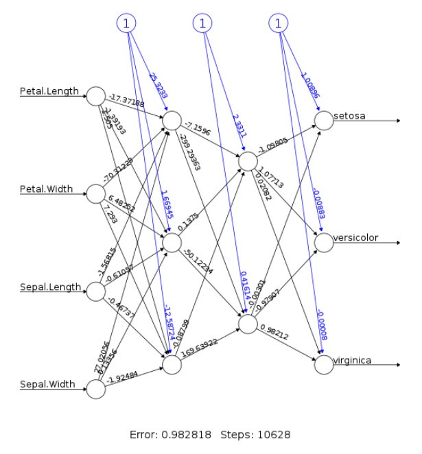
Sample code for trying out this neural network is available in this git hub link.
Extensions and variants
One of the recent extensions of the neural network is the area of deep learning. One of the main feature of deep learning is having a large number of hidden layers.
The implication of large numbers of hidden layers is the possibility of bringing in nonlinear forms of the inputs. Moreover, every one of the hidden layers acts as an input to the subsequent layers. Hence, the nonlinear forms of all these layers are brought into the model making it consume all these data to come out with the best possible model.
Another important aspect of deep learning is that unlike a typical neural network it can learn in an unsupervised mode as well. Which can start learning the data, even before getting the labeled data?
The neural network has evolved into different variants as well. Following are some of the variants,
- Feed forward network: Simple form where the data flows in only in one direction.
- Recurrent neural network (RNN): Unlike feed forward network, here, data flows in both directions. Propagates data from later stages to earlier stages.
- Stochastic neural network: Introduces random variations into the network. It has found some applications in the field of risk management, bioinformatics, etc.
- Convolutional neural network (CNN): Is a form of neural network where the connectivity pattern between the neurons is inspired by the visual cortex of animals. By the nature of it has found useful applications in the area of image processing, visual recognition, etc.
An extensive list of variants can be found in this wiki link.
Deep learning versus wide learning has been one of the recent research topics in this area as well. Wide learning is essentially about adding the capability of generalizing the deep learning models for more use cases and applications.
Hopefully, some level of basic understanding of neural network can be a key take away from this article.