In this article we’ll explore a neat way of visualizing your MP3 music collection. The end result will be a hexagonal map of all your songs, with similar sounding tracks located next to each other. The color of different regions corresponds to different genres of music (e.g. classical, hip hop, hard rock). As an example, here’s a map of three albums from my music collection: Paganini’s Violin Caprices, Eminem’s The Eminem Show, and Coldplay’s X&Y.
To make things more interesting (and in some cases simpler), I imposed some constraints. First, the solution should not rely on any pre-existing ID3 tags (e.g. Arist, Genre) in the MP3 files—only the statistical properties of the sound should be used to calculate the similarity of songs. A lot of my MP3 files are poorly tagged anyways, and I wanted to keep the solution applicable to any music collection no matter how bad its metadata. Second, no other external information should be used to create the visualization—the only required inputs are the user’s set of MP3 files. It is possible to improve the quality of the solution by leveraging a large database of songs which have already been tagged with a specific genre, but for simplicity I wanted to keep this solution completely standalone. And lastly, although digital music comes in many formats (MP3, WMA, M4A, OGG, etc.) to keep things simple I just focused on MP3 files. The algorithm developed here should work fine for any other format as long as it can be extracted into a WAV file.
Creating the music map is an interesting exercise. It involves audio processing, machine learning, and visualization techniques. The basic steps are as as follows:
1. Convert MP3 files to low bitrate WAV files.
2. Extract statistical features from the raw WAV data.
3. Find an optimal subset of these features such that songs which are “close” to each other in this feature space also sound similar to the human ear.
4. Use dimension reduction techniques to map the feature vectors down to two dimensions for plotting on an XY plane.
5. Generate a hexagonal grid of points then use nearest neighbor techniques to map each song in the XY plane to a point on the hexagonal grid.
6. Back in the original high-dimensional feature space, cluster the songs into a user-defined number of groups (k=10 works well for visualization purposes). For each cluster, find the song closest to the cluster center.
7. On the hexagonal grid, color the songs corresponding to the k cluster centers with different colors.
8. Interpolate the colors for other songs based on their proximity in the XY plane to each cluster center.
Let’s look at some of these steps in more detail. To read more click here.
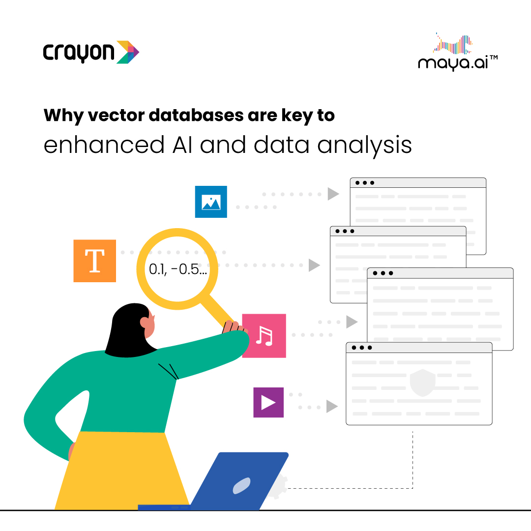
Why vector databases are key to enhanced AI and data analysis
In a...